Propagate through a single-ring antiresonant fibre#

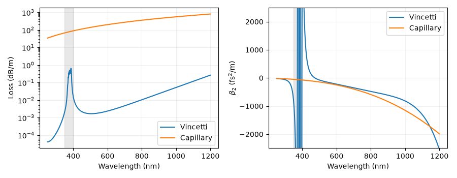
Compare an evacuated 30 um diameter core with a capillary of the same radius. The tube lattice has six tubes of 9 um outer radius and 180 nm wall thickness. The 350-400 nm shaded interval marks the nominal first wall-resonance band; it is a visual guide, not a fitted validity boundary. The plots span 250-1200 nm.

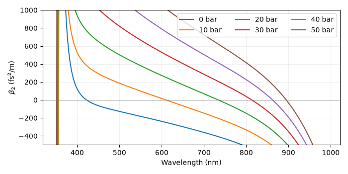
Pressure tuning uses a second geometry: 15 um core radius, 160 nm walls, 6 um outer tube radius and eight tubes, with argon at 0, 10, 20, 30, 40 and 50 bar. All materials use their solprop defaults and the gas is at 293.15 K.

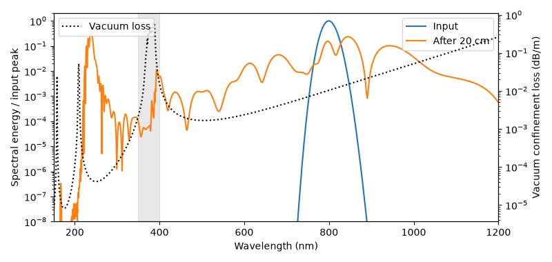
Finally a 1 uJ, 30 fs intensity-FWHM pulse at 800 nm propagates for 20 cm in 5 bar argon in the first fibre, where it self-compresses and emits a resonant dispersive wave near 200 nm, beyond the first wall resonance. The single-mode field grid spans 150-1600 nm and 1 ps, with eight radial nodes and 201 save planes. Kerr and photoionisation are enabled; Raman and third-harmonic generation are disabled. The relative stepping tolerance is 1e-5. Light near the wall resonance has a group delay that no modest window holds, so the temporal collar removes about 2e-5 of the launch energy and warns; the fibre’s loss takes 14 %. This single-mode calculation shows the emission and the transmission window; it is not a converged broadband prediction.

Both geometries extrapolate the published t/r validation range (0.05-0.2), so construction logs a warning. On a fibre of this wall ratio the model’s first-band beta_2 is 20-70 % less negative than a converged finite-element solution’s, so the pressure-tuning curves show the trend with pressure, not a validated beta_2. The vacuum loss overlaid on the 1 bar propagation is within 1 % of the filled fibre’s except on the resonance flank, where the fill moves the resonance by 0.08 nm. The argon index comes from optmat, whose fit covers the whole spectral grid of the propagation, so no material-range warning is raised. The fitted area is available separately; propagation uses Marcatili’s field area.

from time import perf_counter

import matplotlib.pyplot as plt
import numpy as np

from solprop.constants import C
from solprop.driver import prop_capillary
from solprop.log import NullReporter
from solprop.modes import MarcatiliMode, TubeLattice, VincettiMode
from solprop.modes.base import beta2, db_per_m
from solprop.processing.axes import grid_of

started = perf_counter()
lattice = TubeLattice(180e-9, 9e-6, 6)
tube = VincettiMode(15e-6, lattice=lattice)
capillary = MarcatiliMode(15e-6)
wavelength = np.linspace(250e-9, 1200e-9, 600)
omega = 2 * np.pi * C / wavelength

The fitted tube resonances change both attenuation and dispersion. The loss uses the power coefficient; no imaginary-index factor of two is added.

figure, axes = plt.subplots(1, 2, figsize=(9, 3.5))
for mode, label in [(tube, "Vincetti"), (capillary, "Capillary")]:
    axes[0].semilogy(wavelength * 1e9, db_per_m(mode, omega), label=label)
    axes[1].plot(wavelength * 1e9, beta2(mode, omega) * 1e30, label=label)
for axis in axes:
    axis.axvspan(350, 400, color="0.7", alpha=0.3)
    axis.set_xlabel("Wavelength (nm)")
    axis.grid(alpha=0.2)
    axis.legend()
axes[0].set_ylabel("Loss (dB/m)")
axes[1].set(ylabel=r"$\beta_2$ (fs$^2$/m)", ylim=(-2500, 2500))
figure.tight_layout()

Gas pressure changes the material contribution while tube geometry stays fixed.

tuning_lattice = TubeLattice(160e-9, 6e-6, 8)
tuning_wavelength = np.linspace(350e-9, 990e-9, 300)
tuning_omega = 2 * np.pi * C / tuning_wavelength
figure, axis = plt.subplots(figsize=(7, 3.5))
for pressure in (0.0, 10.0, 20.0, 30.0, 40.0, 50.0):
    mode = VincettiMode(15e-6, "Ar", pressure, lattice=tuning_lattice)
    axis.plot(
        tuning_wavelength * 1e9,
        beta2(mode, tuning_omega) * 1e30,
        label=f"{pressure:g} bar",
    )
axis.axhline(0, color="0.5", linewidth=0.8)
axis.set(xlabel="Wavelength (nm)", ylabel=r"$\beta_2$ (fs$^2$/m)", ylim=(-500, 1000))
axis.legend(ncol=3)
axis.grid(alpha=0.2)
figure.tight_layout()

Overlay the propagated spectrum with the fibre’s loss curve. Spectral energy per wavelength includes the omega-to-wavelength Jacobian before normalisation.

output = prop_capillary(
    15e-6,
    0.2,
    "Ar",
    5.0,
    lattice=lattice,
    wavelength=800e-9,
    wavelength_limits=(150e-9, 1600e-9),
    trange=1e-12,
    fwhm=30e-15,
    energy=1e-6,
    envelope=False,
    modes=1,
    kerr=True,
    plasma=True,
    raman=False,
    thg=False,
    n_r=8,
    n_save=201,
    rtol=1e-5,
    progress=NullReporter(),
    seed=20261027,
)
frequency = grid_of(output).omega
active = frequency > 0
spectral_wavelength = 2 * np.pi * C / frequency[active]
order = np.argsort(spectral_wavelength)
spectra = abs(output["field"][[0, -1], 0, 0, :][:, active]) ** 2
spectra = spectra * (2 * np.pi * C / spectral_wavelength**2)[None, :]
spectra = spectra / np.max(spectra[0])
figure, axis = plt.subplots(figsize=(8, 3.8))
for spectrum, label in zip(spectra, ("Input", "After 20 cm"), strict=True):
    axis.semilogy(spectral_wavelength[order] * 1e9, spectrum[order], label=label)
axis.axvspan(350, 400, color="0.7", alpha=0.3)
axis.set(
    xlabel="Wavelength (nm)",
    ylabel="Spectral energy / input peak",
    xlim=(150, 1200),
    ylim=(1e-8, 2),
)
axis.legend(loc="upper right")
loss_axis = axis.twinx()
broad = np.linspace(150e-9, 1200e-9, 900)
loss = db_per_m(tube, 2 * np.pi * C / broad)
loss_axis.semilogy(broad * 1e9, loss, "k:", label="Vacuum loss")
loss_axis.set_ylabel("Vacuum confinement loss (dB/m)")
loss_axis.legend(loc="upper left")
figure.tight_layout()
print(f"Complete Vincetti example: {perf_counter() - started:.3f} s")

BoundaryWarning: the temporal collar removed 1.88e-05 of the launch energy, whose square root is above the 1e-03 budget: what left the window may have mattered; widen trange to keep it
Complete Vincetti example: 3.305 s

Propagate through a single-ring antiresonant fibre#

Related reading#