A line beam under the Kerr effect

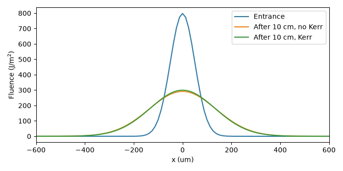
A LineGrid resolves one transverse direction: the beam is uniform in y, so its energy is per metre of y. Here a 100 um waist line of 0.1 J/m, at 800 nm and 30 fs, diffracts through 10 cm of argon at 1 bar. Without the Kerr response its width follows the Gaussian diffraction law; with it, the Kerr lens narrows it slightly.

The first run is a plain prop_free(), every argument an object a recipe writes as a table: Recipe.example("line_beam") is that run.

The launch of the line soliton tutorial is an array, which a recipe does not hold. This one is a SpatialPulse.

import matplotlib.pyplot as plt
import numpy as np

from solprop.driver import SimulationSettings, prop_free
from solprop.grid import EnvelopeGrid, LineGrid
from solprop.nonlinear.responses import KerrResponse
from solprop.physdata import gamma3
from solprop.processing import fluence_map
from solprop.pulses import GaussianPulse, SpatialPulse
from solprop.spatial import SpatialMedium
from solprop.stats import StatsSpec
from solprop.stepper import PIController

WAVELENGTH = 800e-9
"""Carrier wavelength, m."""

WAIST = 100e-6
"""Beam waist, m."""

LENGTH = 0.1
"""Propagation length, m."""

'Propagation length, m.'

The run, with the Kerr response and then without it. The half-width is sixteen waists, so the diffracted beam stays far from the edge of the window.

grid = EnvelopeGrid.from_limits(
    LENGTH, WAVELENGTH, (600e-9, 1100e-9), 200e-15, thg=False
)
space = LineGrid(1.6e-3, 256)
argon = SpatialMedium("Ar", pressure=1.0)
settings = SimulationSettings(
    controller=PIController(rtol=1e-5, atol=1e-12),
    save_planes=[0.05, 0.1],
    dz_init=1e-3,
    dz_max=5e-3,
    stats=StatsSpec(names=("energy", "beam_radius")),
)
beam = SpatialPulse(
    GaussianPulse(wavelength=WAVELENGTH, fwhm=30e-15, energy=0.1), WAIST
)
kerr = prop_free(
    grid,
    space,
    argon,
    [KerrResponse(gamma3("Ar", wavelength=WAVELENGTH), thg=False)],
    beam,
    settings=settings,
    noise=None,
)
linear = prop_free(grid, space, argon, [], beam, settings=settings, noise=None)

The width of the fluence, against the Gaussian law w(z) = w0 sqrt(1 + (z / z_R)^2) with z_R = pi w0^2 / lambda. fluence_map() reads each plane on its transverse axis.

def width(output, plane):
    """Return the second-moment width ``2 sqrt(<x^2>)`` of one plane's fluence, m."""
    profile = fluence_map(output, plane)
    x = profile.axes[0]
    return 2 * np.sqrt(np.sum(profile.fluence * x**2) / np.sum(profile.fluence))


rayleigh = np.pi * WAIST**2 / WAVELENGTH
expected = WAIST * np.sqrt(1 + (LENGTH / rayleigh) ** 2)
print(f"Gaussian law  {expected * 1e6:.2f} um")
print(f"without Kerr  {width(linear, -1) * 1e6:.2f} um")
print(f"with Kerr     {width(kerr, -1) * 1e6:.2f} um")

Gaussian law  273.58 um
without Kerr  273.62 um
with Kerr     267.81 um

The fluence across the line at the entrance and after 10 cm, in J/m^2.

figure, axis = plt.subplots(figsize=(7, 3.5))
entrance = fluence_map(kerr, 0)
axis.plot(entrance.axes[0] * 1e6, entrance.fluence, label="Entrance")
for output, label in ((linear, "After 10 cm, no Kerr"), (kerr, "After 10 cm, Kerr")):
    profile = fluence_map(output, -1)
    axis.plot(profile.axes[0] * 1e6, profile.fluence, label=label)
axis.set(xlabel="x (um)", ylabel="Fluence (J/m$^2$)", xlim=(-600, 600))
axis.legend()
figure.tight_layout()

plt.show()